 Time complexity helps us understand how the running time of an algorithm increases as the size of the input (often denoted as 'n') gets larger. It's a way to predict how efficient an algorithm will be for big problems, without worrying about the exact hardware or small details.
This is expressed using Big O notation, which focuses on the worst-case scenario – the maximum time an algorithm might take for a given input size. Big O gives us an upper bound on the growth rate, ignoring constant factors and smaller terms to focus on the big picture.
Here are some common Big O notations, explained with examples:
O(1): Constant time
The algorithm takes the same amount of time no matter how large the input is. For example, accessing a single element in an array by its index – it's instant, like picking a book from a shelf when you know exactly where it is.
O(n): Linear time
The time grows directly with the input size. For instance, looping through a list to find the maximum value – if the list doubles in size, the time roughly doubles, like checking each page in a book one by one.
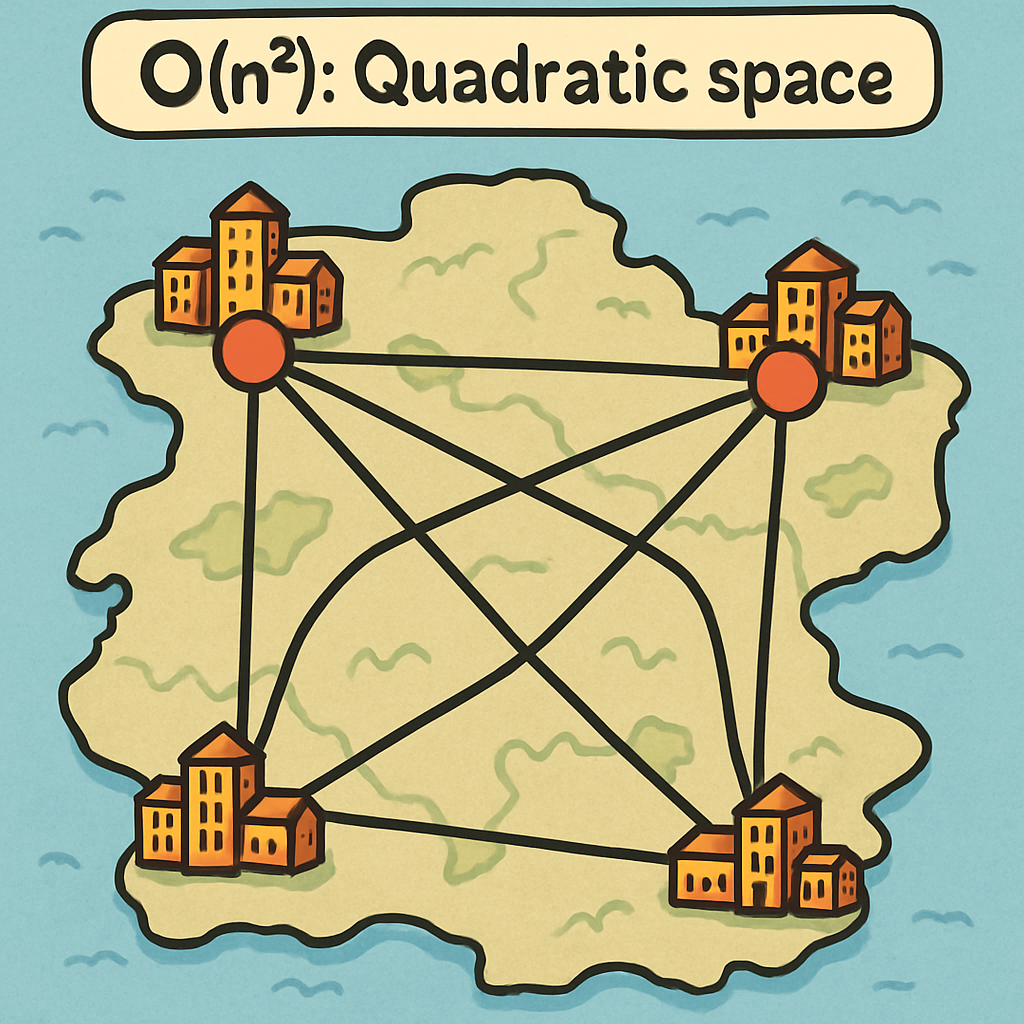
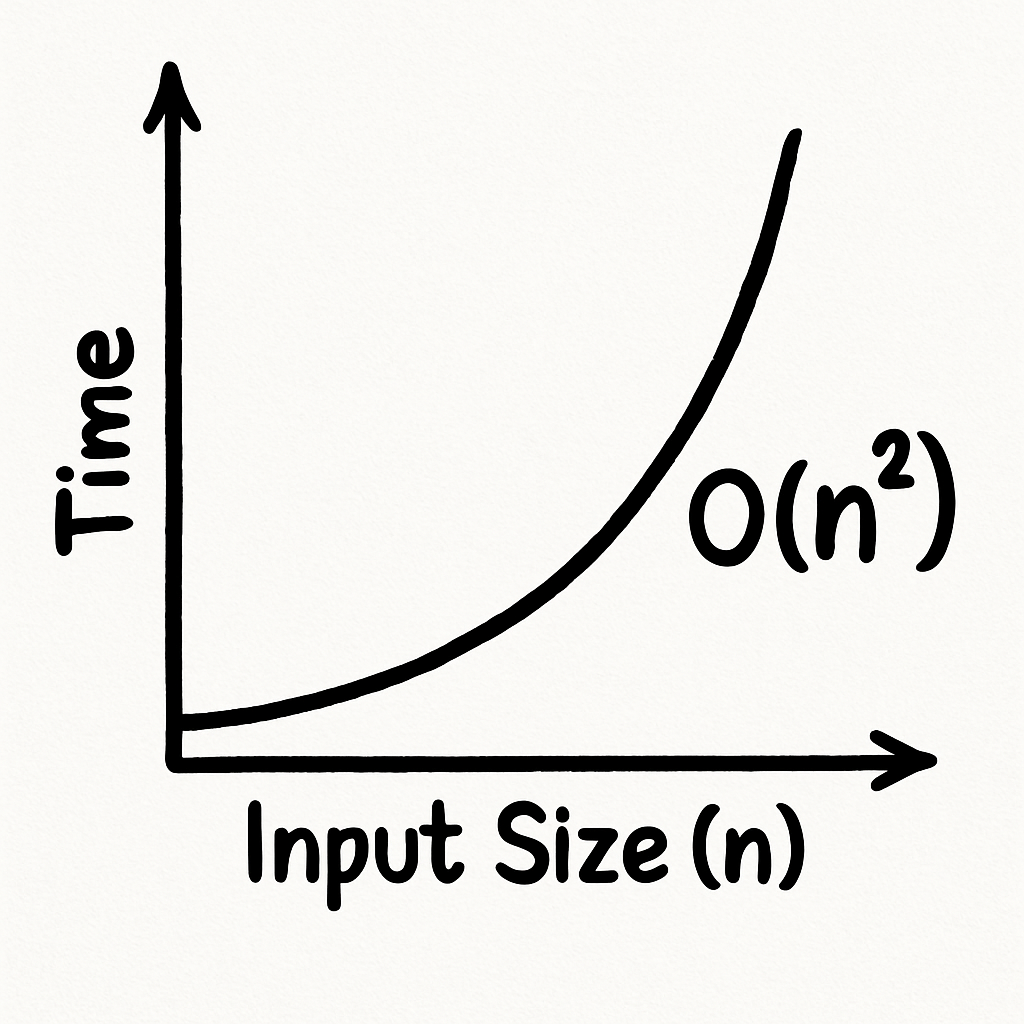
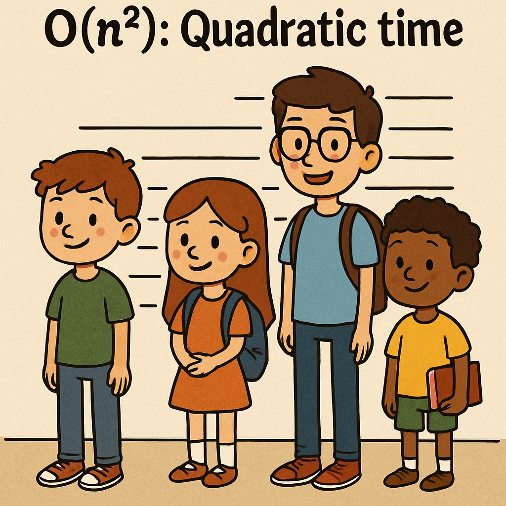
O(n²): Quadratic time
This often happens with nested loops, where for each item, you check every other item. Bubble sort is a classic example – for large lists, it can be very slow because if n doubles, the time quadruples (since (2n)² = 4n²). Imagine comparing every pair of students in a class to sort them by height; with twice as many students, you'd have four times as many comparisons.
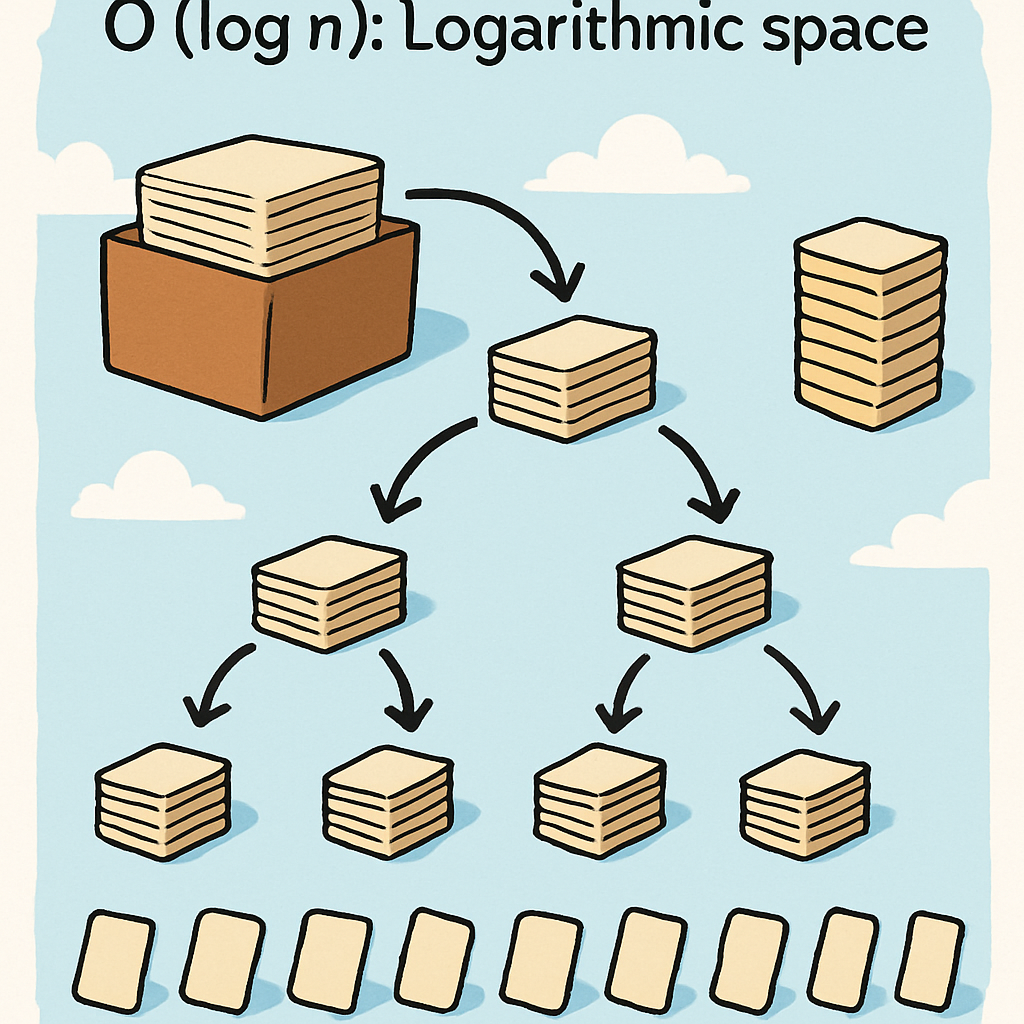
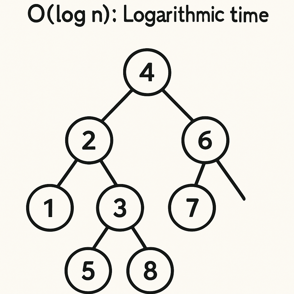
O(log n): Logarithmic time
The time grows very slowly as n increases, often seen in divide-and-conquer strategies. Binary search on a sorted list is a great example – it halves the search space each step, so for a list of a million items, it might only take about 20 steps. It's like guessing a number between 1 and a million by repeatedly asking if it's higher or lower – you narrow it down quickly.
In sorting algorithms, bubble sort has a time complexity of O(n²) because of its nested loops, making it inefficient for large datasets. Quicksort, on the other hand, has an average time complexity of O(n log n), which is much better – it grows slower than quadratic but faster than linear.
Remember, Big O simplifies things by ignoring constants and less dominant terms to focus on the overall growth rate as the input size becomes very large. For example, if an algorithm's time is described by 3n² + 2n + 1, we drop the constant 3 (so it's just n²), and ignore the 2n and +1 terms, leaving O(n²). This is because as n gets really big – say n=1000 – the n² term (1,000,000) dominates over 2n (2000) and the constant (1), which become negligible in comparison.
Constants are ignored because whether it's 3n² or 5n², both grow at the same rate category; it's the n² that defines the behaviour for large n. Think of it like comparing the speed of cars on a long journey – the top speed matters more than whether one has a slightly better acceleration from a stop.
Understanding Big O helps you choose the right algorithm for the job, especially when dealing with large amounts of data.
 Chromebooks, laptops, and PCs are crucial tools for coding and digital skills education. Chromebooks are ideal for web-based applications and collaborative projects, while laptops and PCs support a wider range of programming environments and software for more intensive tasks like software development and data analysis.
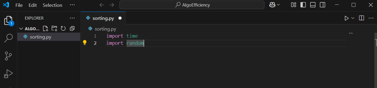
 In this lesson you'll learn about time and space complexity, Big O notation, and apply these concepts by implementing and timing sorting algorithms in Python using VS Code.
 Algorithmic efficiency refers to how well an algorithm performs in terms of time (how fast it runs) and space (how much memory it uses). Efficient algorithms solve problems quickly and with minimal resources, which is crucial for large datasets, such as those in social media apps or scientific simulations where speed and low resource use can make a big difference.
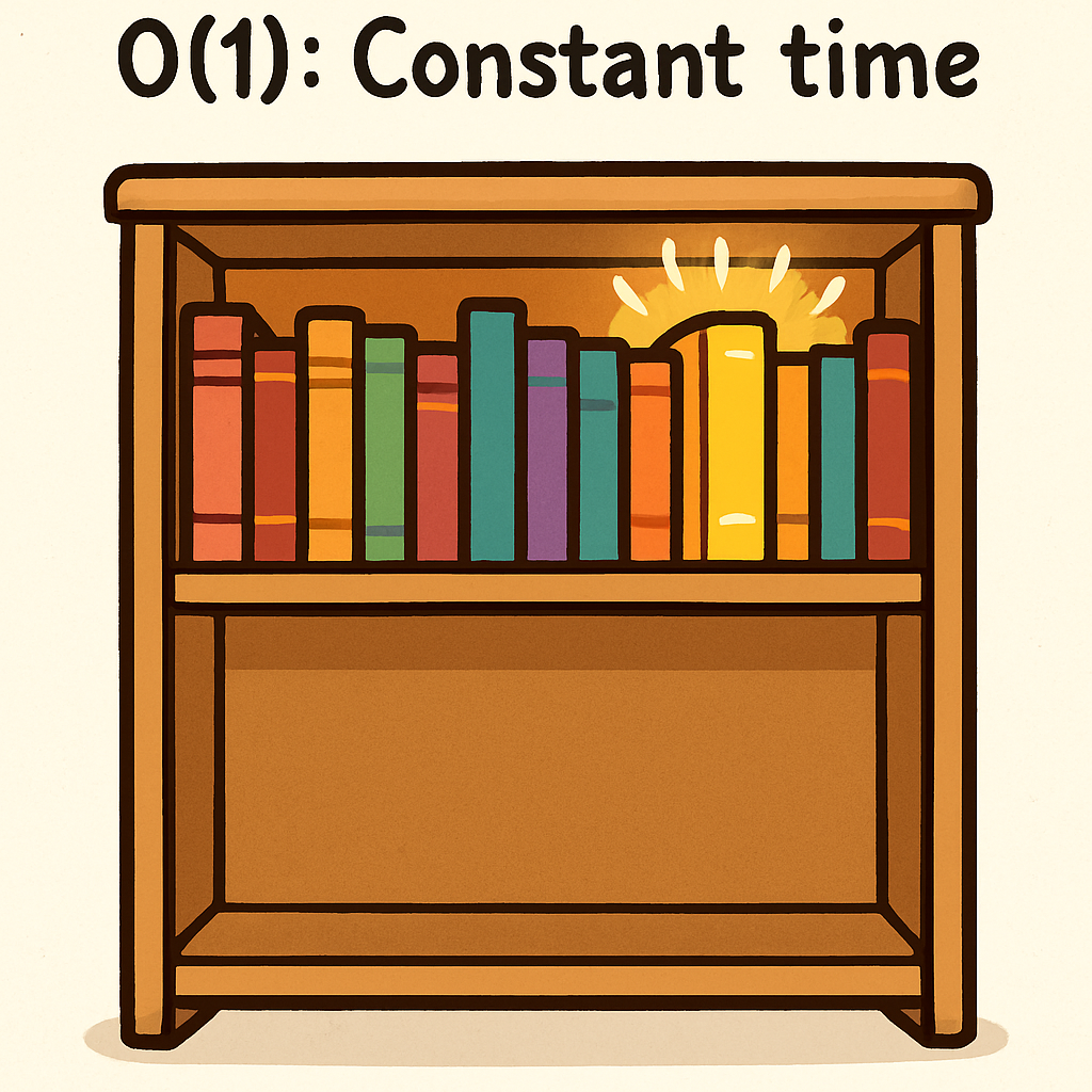

 Space complexity measures how the memory usage of an algorithm increases as the size of the input (often denoted as 'n') gets larger. Just like time complexity, it's expressed using Big O notation, focusing on the worst-case scenario – the maximum memory an algorithm might require for a given input size.